Existence and uniqueness theorems for 1st-order ODE
The general 1st-order initial value problem (IVP) is $$\begin{equation}\tag{*}y’=F(x,y), y(x_0) = y_0.\end{equation}$$ We are interested in the following questions:
- Under what conditions can we be sure that a solution to (*) exists?
- Under what conditions can we be sure that there is a unique solution to (*)?
Here are the answers.
Theorem (Existence and uniqueness). Suppose that F(x,y) is a continuous function defined in some region $$R = (x_0-\delta, x_0+\delta)\times (y_0-\epsilon, y_0+\epsilon)$$ containing the point (x_0, y_0). Then there exists \delta_1 > 0 so that a solution y=f(x) to (*) is defined for x\in (x_0-\delta_1, x_0+\delta_1). Suppose, furthermore, that \frac{\partial F}{\partial y}(x,y) is a continuous function defined on R. Then there exists \delta_2 > 0 so that the solution is the unique solution to (*) for x\in (x_0-\delta_2, x_0 + \delta_2).
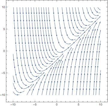
Example 1 Consider the IVP y'=x-y+1, y(1)=2. In this case, both the F(x,y)=x-y+1 and \frac{\partial F}{\partial y}(x,y)=-1 are defined and continuous at all points. The theorem guarantees that a solution to the ODE uniquely exists in some open interval centered at 1. In fact, an explicit solution to this equation is y(x) = x+e^{1-x}. This solution exists for all x.
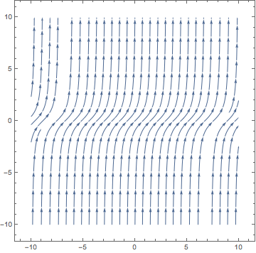
Example 2 Consider the IVP y' = 1+y^2, y(0)=0. Both F(x,y)=1+y^2 and \frac{\partial F}{\partial y}(x,y)=2y are defined and continuous at all points, so by the theorem we can conclude that a unique solution exists in some open interval centered at 0. By separating variables and integrating, we derive a solution to this equation y(x)=\tan x. Remember that a solution to a DE must be a continuous function! In order for this function to be considered as a solution to this IVP, we must restrict the domain to x\in (-\pi/2,\pi/2).
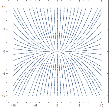
Example 3 Consider the IVP y' = 2y/x, y(x_0)=y_0. In this example, F(x,y) = 2y/x and \frac{\partial F}{\partial y}(x,y)=2/x. Both functions are defined for all x\neq 0, so the theorem tells us that for each x_0 \neq 0 there exists a unique solution in an open interval around x_0. By separating variables and integrating, we derive solutions y(x) = Cx^2 for some constant C. Notice that all of theses solutions pass through (0,0). So the IVP y'=2y/x, y(0)=0 has infinitely many solutions, but the IVP y'=2y/x, y(0)=y_0\neq 0 has no solutions.